Upsolver Self-Guided SQLake Hands-On Labs

Welcome to Upsolver SQLake

SQLake is ...

The initial lab will take around 20 minutes, and includes a general walkthrough, a brief tour of the user interface, and creation of your first pipeline. From there, you can continue on to additional labs will walk you through the power of Upsolver's streaming ETL capabilities along with it's Kappa architecture.

The Kappa architecture has several benefits:

• Handle all batch and streaming use cases with a single architecture (say "no" to Lambda architecture)
• One codebase that is always in sync
• One set of infrastructure and technology
• The infrastructure is near real-time, scalable, reliable (idempotent), and cost effective
• Improved data quality with guaranteed ordering and no mismatches (exactly-once processing guarantee)
• No need to re-architect for new use cases

At the end of each lab, we will propose some additional self-guided exercises that you may complete if you wish to expand your learning of Upsolver.

---

Let's Get Started - Sign-up

Navigate to the sign-up page, and click the 'Sign Up' link at the bottom of the Log in window.

---

Exercise 1

Now lets build our first pipeline. In this pipeline, we are going to be taking some streaming data from an S3 bucket that Upsolver provides. We will ingest that raw data into a staging table, where we store an immutable copy of it in its raw form, catalog its structure and metadata, and make it accessible for querying and downstream processing. We will then create a series of transformations on this raw data, and query that transformed data with Athena.

Upon first login, you are presented with an introduction to the platform. Feel free to step through the wizard until you get to the “Done” button.

When you finish the initial wizard you are presented with a set of out of the box templates. These templates can serve as introductions to common pipeline use cases that you may wish to explore. The “Templates with Sample Data” section, include everything that you need to build a full end to end pipeline, and is where we will start. The other templates provided will require you to connect to your own data sources, i.e. Kinesis or Kafka, streams, but include example scripts and commands to work with whatever data that you have available. In this lab, we are going to start with the S3 to Athena (sample data) template.

UI walkthrough

Before we get into the template itself, lets walk through the core components of the UI.

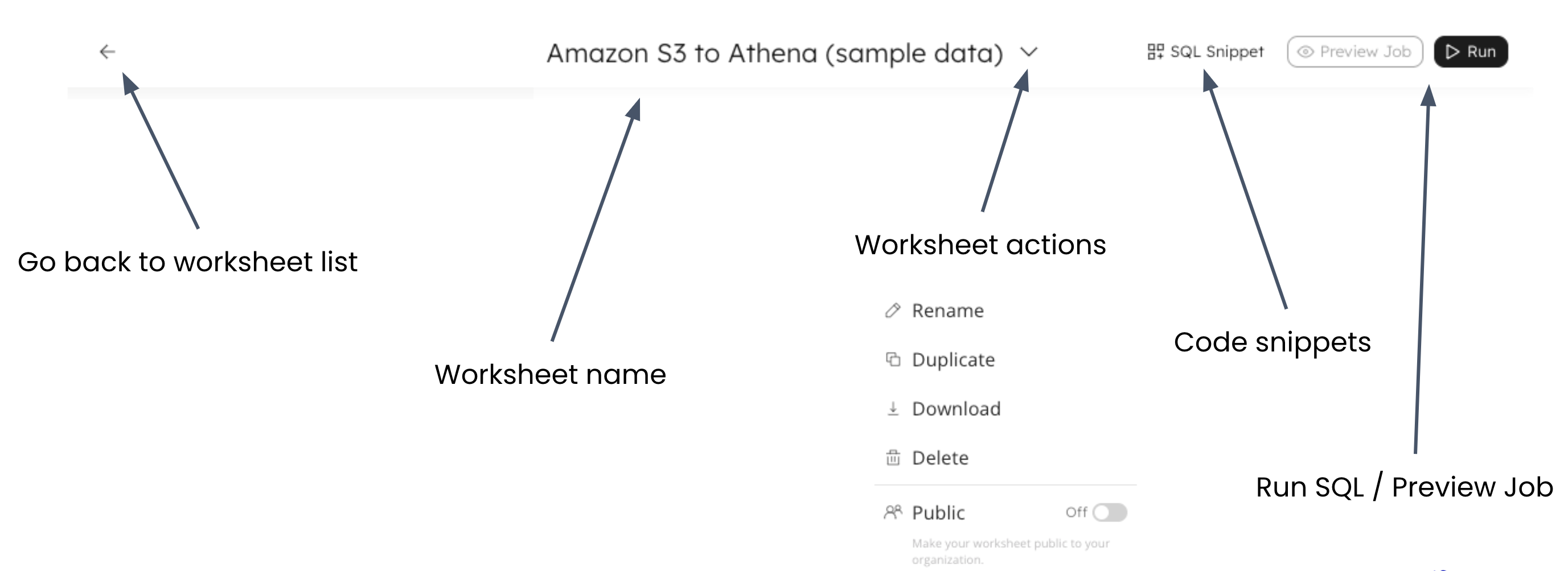
There is a back button in the upper left hand corner of the screen that you can use to go back to your worksheets list, choose a different template to work with, or navigate to other sections of the SQLake UI.

The center of the title bar shows you the worksheet that you are currently working with. This current worksheet was based on the template that we chose. The down arrow next to the worksheet name provides a menu that allows you to rename your worksheet, duplicate it (often used to create backup copies), download your worksheet as a SQL file, delete your worksheet, or make it public. Worksheets are private by default, only visible to you, but if you have multiple users in the same organization, you can share worksheets with others by making them public.

Continuing to the right, there is a SQL Snippet button to include common code blocks into your worksheet, and finally a “Preview Job” and “Run” button that we will see in action later in the workshop.

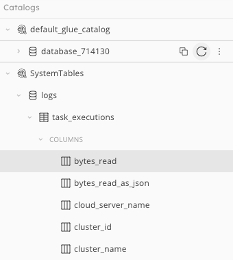
Catalog - Displays available connections
* By default, every user has two connections Types of connections * GLUE_CATALOG * S3 * KINESIS * KAFKA * SNOWFLAKE

Help and documentation
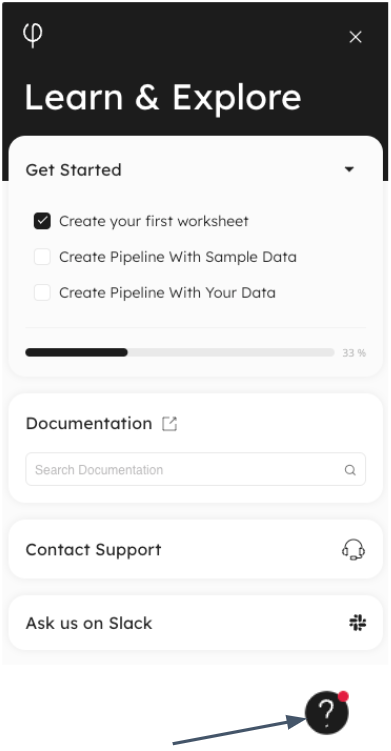	* Searchable documentation * Ask general questions on Slack * Contact support if something doesn’t work as expected

Our Sample Data
The sample data that we will use throughout this exercise is streaming orders data from a fictional e-commerce website. We are working as data engineers and being asked to transform this data for a variety of purposes while populating a data lake for historical reporting

Take a look at your Worksheet (Template)

Step 1: Create connection to S3

/*
   1. Create an S3 connection to manage IAM credentials for jobs that need to access data in S3
*/
CREATE S3 CONNECTION upsolver_s3_samples
   AWS_ROLE = 'arn:aws:iam::949275490180:role/upsolver_samples_role'
   EXTERNAL_ID = 'SAMPLES'
   READ_ONLY = TRUE;

To run a command: Place your cursor within the command and click the Run button in the upper right Click the + button to the left of the line number, and select “Run Statement” Press a keyboard shortcut (i.e. on Mac or on Windows

Browse Newly Created Connection

With your connection created, you will see it appear in the catalog view on the left. Browse through the connection, noticing the bucket/folder structure of the sample data.

Step 2: Create a staging table for data ingestion

With our source connection created, scroll down to Step 2 in the worksheet, where we will create our staging table to load our raw data into. Creating this table is as simple as giving your table a name, and choosing how you want your data to be partitioned. We do not have to define the full schema of the table, as it will be built out as streaming data is ingested.

In most use cases, staging tables will be partitioned by the $event_date system column, which is the timestamp of when the incoming event was processed.

/*
   2. Create an empty table to use as staging for the raw data.
*/
CREATE TABLE default_glue_catalog.database_714130.orders_raw_data()
   PARTITIONED BY $event_date;

Go ahead and run this command, and view your newly created staging table in the catalog view.

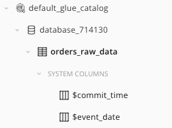
View Your Table in the Catalog

Notice that since your table is empty, there are no columns, other than two system columns.

Step 3: Create your ingestion job

A COPY FROM job takes data from a source connection, and loads it into a staging table. This job instructs SQLake to ingest data from our S3 source, and write it into our staging table.

/*
   3. Ingest raw data from your bucket into the staging table
*/
CREATE JOB load_orders_raw_data_from_s3
   CONTENT_TYPE = JSON
   AS COPY FROM S3 upsolver_s3_samples BUCKET = 'upsolver-samples' PREFIX = 'orders/'
   INTO default_glue_catalog.database_714130.orders_raw_data;

we are defining the incoming CONTENT_TYPE as JSON. Upsolver supports many common data types such as JSON, CSV, TSV, AVRO, PARQUET, XML, ORC, etc…

The BUCKET and PREFIX parameters simply tell the ingestion job where to find the incoming data within the provided S3 connection.

All other parameters are left as default, with a full list available in the documentation. Parameters exist to tell the ingestion job how the ingested data is partitioned at the source, whether the data is compressed or not, and how far back in time to ingest the data.

Notice the COPY FROM syntax within the job. There are other types of jobs that we will create later in this workshop depending on what action the job is taking.

Musical Interlude

While your job begins to ingest and process data, let's take a minute just to explain a little about what’s happening behind the scenes:

• SQLake is ingesting raw S3 files a breaking them down minute-by-minute in a micro-batch, or stream-based process.
• As data is ingested and processed, standard Parquet files are being created in the target S3 bucket where you defined your staging table.
• These files are partitioned by date (default configurable), and continuously compacted in the background for efficient, optimized downstream use.
• As data is being ingested, SQLake is also identifying and storing statistics and metadata that describe the incoming data, which we can take a look at to assist in building out transformations.

Refresh the table to see data columns	Click on the table name, and expand the properties pane

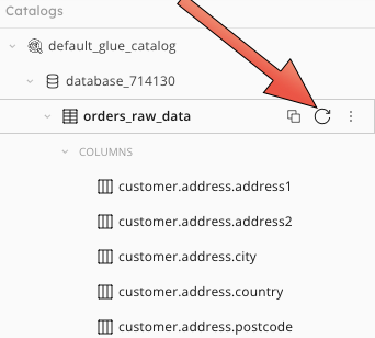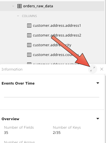With the table selected, the right hand pane will show an events over time graph, along with some high level overview metrics

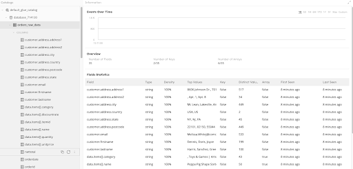
Scrolling down you can see a list of ingested fields. SQLake has automatically inferred the data type of the incoming data, along with its density (how often it shows in each event), cardinality, top values, and when that field was first and last seen. This is especially useful as schema’s evolve overtime. In our example you can see that all fields were first and last scene at the same time. If we run this ingestion over the next few months though, if a new field starts showing up in our data we may see that data was first seen a few days ago, or we may see that a field was last seen a few days ago. Keeping tabs on this will help us know whether we may want to include, or exclude certain fields in our transformations, and/or update our transformations as our schema evolves.

Now click on a specific field in the left hand catalog view, for example customer.address.state. The field details will show some key overview metrics, but also give you a sampling of values that we’ve seen, along with their distribution within the data.

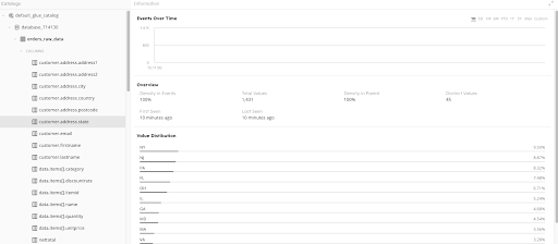
Click through several fields and take note of any data “problems” that you see, for example 0 showing up in the nettotal column and the ordertype field having both upper and lower case values.

Because SQLake is directly integrated with Amazon Athena, you can directly query your ingestion table from within a worksheet. This is useful for verifying that data is being properly ingested, as well as for inspecting whether certain fields are as you expect. Go ahead and run the SELECT * in the worksheet, and see how the result set appears in your worksheet. Note: it make take 3-4 mins for data to populate the table.

/*
   Query your raw data in the staging table
   Note: It may take 3-4 minutes for the data to appear in your staging table.
*/
SELECT * FROM default_glue_catalog.database_714130.orders_raw_data limit 10;